Building a persistent BEV traversability map, and the four things its scalar metric refused to see
Building a persistent BEV traversability map, and the four things its scalar metric refused to see
Part of the Terra Perceive series.
The previous milestone shipped a pose-graph SLAM stack that produced metric-grade trajectories on RELLIS-3D and a covariance estimate per pose. The optimizer’s posterior was correct. Nothing in the project actually consumed it. This milestone is the one where the pose graph’s output finally lands somewhere useful: a persistent bird’s-eye-view map that fuses 2,847 LiDAR scans into one risk grid, weights each observation by the SLAM uncertainty at that frame, and publishes the result over a real message broker so that the next milestone’s tracker can subscribe.
Three things happened along the way that the post is honest about. The first is that the trajectory paints itself bright yellow in every map I produced, which looks like a bug, is not a bug, and is in fact the standard failure mode of geometric ground segmentation in unstructured off-road environments. The second is that I picked the wrong scalar metric on the way in: coverage-ratio, the headline number I designed the eight ablations around, turned out to be blind to the things I was ablating. The five thousand lines of CSV the runs produced still tell a real story, but the story is qualitative and lives in the per-cell time-series plots. The third is the NATS broker hitting its 1 MB default payload limit on the first BEV publish at full resolution, which forced an honest read of the production gap between “transport bootstrap” and “production telemetry.”
The post walks the build, then each of the three honest moments, then the eight ablations briefly, then the transport layer, then what shipped and what did not.
If you are new to occupancy-grid mapping, the early sections are a working tour of the data structure and the three update rules. If you have shipped one of these in production, the value is in the ablations: which knobs the data on this dataset actually responds to, which it does not, and which honest scalar to publish when coverage-ratio refuses to move.
Every claim that follows is reproducible from the artifacts in results/m3/ and the per-frame snapshots on the project’s external drive at /media/nishant/SeeGayt2/terra_perceive/m3_perframe/. Every figure was rendered by a script in scripts/blog_m3/ against those artifacts; no number in this post is hand-edited.
What this builds, and what was already there
The earlier post in this series (m8-slam) shipped the pose graph: a manifold Levenberg–Marquardt optimizer over a graph of ICP, IMU-preintegrated, GPS, and Scan-Context loop-closure edges, with the SLAM trajectory exported as data/poses_slam_manifold.csv. The g2o reference optimizer, retained as a cross-check, produced a near-identical trajectory and exposed a per-pose 6×6 covariance via computeMarginals. Nothing in the rest of the project consumed that covariance.
The single-frame traversability grid from Phase 1 produced a per-frame 0.5-metre BEV grid in the vehicle frame, with one risk value per cell derived from RANSAC-segmented obstacle points. The grid lived for one frame and was discarded. Successive frames did not accumulate evidence about the same physical cell of the world.
The transport layer consisted of a transport/proto/perception.proto file with a BEVGrid message stub and a docker-compose stanza for a NATS broker with the --jetstream flag, both inherited from earlier scaffolding. Neither produced a single byte on the wire.
The deliverable for this milestone is the joined system: a persistent world-frame grid that consumes the SLAM trajectory and the per-pose covariance, integrates per-frame LiDAR observations under three configurable update rules, downweights observations by SLAM uncertainty when the covariance is available, snapshots the state at each frame, and publishes the resulting BEV grid as a versioned protobuf message on the broker for any consumer that subscribes. Plus the eight ablations that justify each parameter choice. Plus the blog post you are reading.
The pipeline

Per LiDAR frame the pipeline runs end-to-end. RANSAC segments ground from obstacle points. The per-frame TraversabilityGrid turns the obstacle cloud into a vehicle-frame risk grid. The WorldGrid accumulator transforms each cell to the world frame using the SLAM pose, looks up the corresponding world cell, and updates it under the chosen rule. The result is serialized as a BEVGrid protobuf and published on perception.traversability.grid. The dashboard subscribes and renders the grid live; the M4 tracker subscribes when M4 is built.
The grid is 1000 cells on each side at 0.5-metre resolution, which works out to a 500-metre square centred on the world origin. RELLIS sequence 00 ends with the vehicle at world (-208, 119), which fits comfortably inside that square. An earlier version of the WorldGrid used a 200-metre square (centred at the origin and extending only to ±100 m), and the vehicle drove off the grid past frame 1500. Observations beyond that point were silently dropped by the bounds check in WorldGrid::worldToGrid. The fix was a one-line config bump after the symptom (the final map looking truncated) was diagnosed; the lesson is that the grid extent has to be sized to the trajectory, not to a default constant. Both lessons (sizing the grid to the data, sanity-checking the cumulative observed-cell bbox) made it into a feedback memory so the next milestone’s animation viewport is not re-derived from scratch.
The covariance branch is optional but on by default in the demo run. If --cov-source g2o is passed, the accumulator loads data/poses_slam_manifold_cov_g2o.csv (a 36-column table with one 6×6 covariance matrix per pose, written by the slam-runner side under a separate flag), computes a scalar pose_sigma = sqrt(trace(P_translation_block)) per frame, and downweights every observation in that frame by exp(-k * pose_sigma) with k=1.0. Section Pose covariance flowing into the map is what this does and why it matters.
The WorldGrid as a data structure
The persistent grid is a flat std::vector<WorldCell> of rows * cols entries indexed [col, row] (the convention here is that the CSV row field indexes the world-x direction and col indexes world-y; this is the opposite of standard image-display convention and required a careful patch in every visualization script that overlays a trajectory on the rendered grid). Each WorldCell carries six fields:
struct WorldCell { float risk = 0.0f; // [0,1] — EMA or sigmoid(logodds) float logodds = 0.0f; // for log-odds rule only float confidence = 0.0f; // [0,1] — observation trust uint32_t obs_count = 0; uint32_t last_update_time = 0; // frame index of last update float mean_z = 0.0f; float pose_sigma_at_last_obs = 0.0f; // for replayability of Ablation E};risk is the headline value the downstream consumer reads. logodds is a side-channel maintained only by the log-odds rule (and ignored by EMA and overwrite). confidence is the per-cell trust accumulated across observations, downweighted by pose_sigma. The remaining fields are diagnostic / replay state: obs_count answers “has this cell been observed at all” and serves as the masking bit for the visualization layer; last_update_time enables the optional temporal-decay rule; mean_z is the running average of LiDAR-return height in the cell; pose_sigma_at_last_obs is the SLAM uncertainty at the frame the cell was most recently updated, persisted so any post-hoc analysis (Ablation E in particular) can reconstruct the confidence weight without rerunning the accumulator.
The grid is serialized in two forms per snapshot. A sparse CSV (snapshots/frame_NNNNN.csv) lists every cell that has been observed at least once, one row per cell, with all six fields. A rendered PNG (final_grid.png plus per-snapshot PNGs) is a viridis-colour-mapped rendering of the risk field. The CSV is the source of truth and is what every figure script in scripts/blog_m3/ reads; the PNG is a thumbnail. The single largest gotcha across this milestone, captured in feedback_diagram_plot_rules.md, is that loading the PNG with naive matplotlib imshow and origin=‘lower’ does not align the heatmap with the trajectory. Always load the CSV.
Three update rules

The accumulator supports three update rules behind a strategy enum, selectable at runtime. The reason for shipping all three rather than picking one early is that the three correspond to three different priors about what an observation means, and the right prior depends on the regime — and on RELLIS sequence 00 the regime turns out not to discriminate between them on any scalar metric I could think of, which is part of the story of the next two sections.
EMA (exponential moving average)
The simplest of the three. On each observation, the cell’s risk value is a convex combination of the new observation and the old state:
with chosen at construction time. This is a one-pole infinite-impulse-response filter; the cell’s effective memory is roughly observations, so smooths over the most recent ~3 observations while keeping the cell responsive to genuine state changes. EMA has no probabilistic interpretation as such — it is a smoothing primitive — but the trade-off it parameterises is exactly the one occupancy mapping cares about: how strongly should a new measurement override the existing belief about a cell.
The ablation in section The alpha sweep walks through how that trade-off plays out on real data. The shipped default of is justified there.
Log-odds (OctoMap-style)
The standard Bayesian-occupancy formulation. Each cell holds a log-odds value that accumulates additively under the assumption that successive measurements are conditionally independent. A “hit” (a measurement implying the cell is occupied) adds a positive increment; a “miss” adds a negative increment; the cell’s risk is then the sigmoid of the accumulated log-odds:
The clamps and are what makes this the OctoMap-style variant rather than naive log-odds [1]. Without them, a long sequence of consistent measurements drives to ±infinity and the cell becomes pinned at risk 0 or 1; the cell can no longer respond to a state change because no finite stream of opposite-sign measurements can move it back. Hornung et al. introduced the clamping policy specifically to keep cells responsive in dynamic environments, and the shipped values are taken directly from the OctoMap reference implementation. The hit/miss increments themselves are derived from the accumulator’s interpretation of the per-frame risk: a new_risk > 0.5 adds the hit increment, otherwise the miss increment. This thresholded version is appropriate for traversability where the per-frame estimate is itself probabilistic but the integration regime favours discrete evidence accumulation.
The principled appeal of log-odds over EMA is the additivity. With independent measurements the log-odds increment is a sufficient statistic; the order of observations does not matter (modulo clamping), and the steady state has a clean Bayesian interpretation. The practical question is whether the additivity actually buys anything on RELLIS, where the per-frame measurements are noisy and not really conditionally independent across the LiDAR sweeps. The ablations spend a lot of words on this.
Overwrite
The trivial rule: each new observation replaces the cell’s risk value entirely. No memory, no smoothing, no probabilistic interpretation.
The reason to ship this rule is not that anyone would deploy it. The reason is that it provides a useful baseline for the other two: any visible difference between a smoothing rule and overwrite is the smoothing rule actually doing work. If EMA at produces a final map that is within visual noise of overwrite, then EMA is buying nothing on this dataset and the shipped default is wrong. Section The update-rule story is qualitative, not scalar is what that comparison actually shows.
The three rules are unified through a tiny strategy interface in include/world_grid.hpp, and the choice is one CLI flag: --update-rule {ema,logodds,overwrite}. The runner mirrors slam_runner.cpp’s pattern exactly, which is the project-wide convention captured in feedback_runner_binary_pattern.
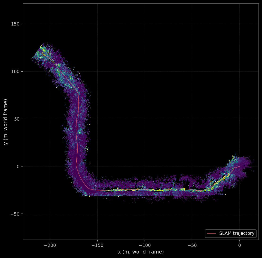
Why the path is bright yellow
The first time I rendered the final map I assumed it was a polarity bug.
The colour bar on every BEV map says yellow is risk = 1 (hazard) and dark is risk = 0 (safe), per ISO 3864 and the project’s feedback_blog_style convention for warning colours. The vehicle drove through the bright yellow region without incident; nothing exploded; no person was harmed; the path is, by any reasonable definition, the most-traversable part of the scene. So the visualization had to be inverted somewhere. I spent an evening trying to find the inversion. It was not there.
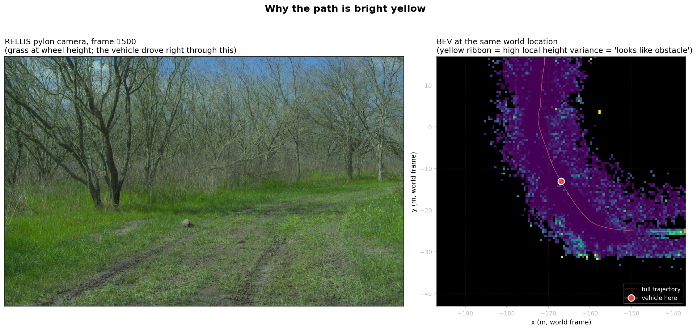
The actual diagnosis. The per-frame TraversabilityGrid computes risk from local height variance: cells whose LiDAR returns span a wide range of get classified high-risk; cells whose returns are coplanar get classified low-risk. This heuristic works in structured environments where obstacles are vertical and ground is flat. In RELLIS sequence 00 the dataset’s defining property is that this heuristic does not work. The ground is not flat. The vehicle is driving through tall grass. Each LiDAR sweep produces returns from grass blade tops, from grass blade bases, from the dirt under the grass, and from the wheels and chassis of the Polaris itself when the sensor’s near-field returns hit them. Per cell, the height variance of those returns is consistently high. The classifier reports those cells as obstacles.
Off-path cells get sparser returns at grazing incidence (the LiDAR sees grass tufts from the side, not from above; one or two beams hit each tuft instead of dozens), the local height variance is lower because each cell sees fewer returns concentrated in the upper-grass region, and the classifier reports those cells as safe. The result is the inverted-looking pattern: the trail the vehicle is driving on is the cell with the densest LiDAR coverage and therefore the highest measured height variance, and the surrounding terrain is sparser and registers as smoother.
The algorithm is doing exactly what it was told to do. What it cannot do, with LiDAR alone, is distinguish 0.5 metres of grass (traversable) from 0.5 metres of cedar bush (not traversable). Both look identical in pure point-cloud geometry. This is the failure mode RELLIS-3D was built to expose. From Jiang et al.’s introduction to the dataset [3]:
Traditional geometric classifiers fail in unstructured off-road environments because vegetation height-variance overlaps the obstacle distribution.
The map’s “yellow path” is the M3 system being honest about its perceptual limit. The fix is semantic segmentation: actually identify “this point belongs to class GRASS” versus “this point belongs to class TREE_TRUNK,” then use the class label to downweight high-variance grass while keeping high-variance bushes risky. The project plan has SegFormer fine-tuning on RELLIS as the P3 stretch milestone, and that is the right place to address it. The current blog refuses to invert the colormap or post-process the path away because doing so would silently lie about what the codebase computes.
The figure pair above is what actually convinced me. Left panel: the camera shows what the scene looked like to a human eye on the day of recording. Right panel: the geometric classifier’s honest report of what it could measure. The two panels disagree, and the disagreement is the project’s strongest motivation for the next milestone’s perceptual upgrade.
The eight ablations and a metric that did not move
The plan called for five ablation axes (pose source, update rule, EMA , temporal decay rate, covariance source), each with a small grid of parameter values, all reported under a single coverage scalar that I expected to move with the parameters being swept. Thirteen runs of accumulator_runner across the four axes (de-duplicating the SLAM-EMA baseline shared between several axes) produced thirteen metrics.json files with thirteen final_coverage numbers. The numbers did not move. The full spread across all thirteen runs is 0.3775 to 0.3852, a range of 0.77%. That is the headline finding of the entire ablation campaign, and the section the rest of the post hangs off.

What coverage is, mathematically: the fraction of cells in the trajectory’s bounding hull that have been observed at least once. Computed each frame, written per-frame to coverage.csv. The intent was to use this as the scalar that distinguishes pose sources (cleaner poses → tighter hull → higher fraction observed), update rules (different rules → different definitions of “observed enough”), and so on.
Why it does not move. Coverage measures only the bitmask of which cells have been observed at least once. Every parameter being ablated affects the value the cell gets updated to, not whether the cell gets touched at all. Two runs with identical poses and LiDAR but different update rules write into exactly the same set of cells; the cells’ final values differ but the bitmask is identical. The same goes for : the EMA filter modifies the value, never the membership. Same for decay: a high decay rate makes cell values fade over time but does not unmask them. Same for covariance source: the downweighting affects confidence values but not the binary “was this cell ever updated” question.
The coverage metric I designed the entire campaign around was, on this regime, structurally blind to four of the five axes I meant to ablate. The only axis it could in principle distinguish (pose source) it does distinguish, but only weakly: the pose sources differ in trajectory shape, which differs in hull shape, which differs in the size of the denominator. The actual ranking the full bitmask produces is carto_ema (0.3852) > gps_ema (0.3840) > slam_logodds (0.3800) > slam_ema (0.3796) > gps_ema (0.3791) > ... > slam_overwrite (0.3775), with all neighbours separated by less than 0.5%. Any one of those numbers would be defensible as the “winner” depending on which decimal place you stop reading at.
Two responses to this. First, the obvious: keep the coverage metric in the audit trail (it is computationally cheap and a useful sanity check that the runs all touched roughly the right number of cells), but stop reporting it as the headline number. Second, the harder one: the actual story this milestone has to tell about update rules, alpha, decay, and covariance is qualitative, and lives in the per-cell time-series plots that the next four sections introduce. Each ablation’s hero figure is now a value-vs-time plot for one carefully-chosen world cell, traced across all the runs in that ablation. The cell selection is documented in scripts/blog_m3/pick_hero_cell.py: the picker reads every snapshot CSV, finds cells that were observed at least 8 times across the run, computes their temporal variance, and ranks by variance / (1 + d_traj/10) where d_traj is the cell’s distance to the nearest trajectory waypoint. The chosen cell is at world (-198, 113.5), near the trajectory’s terminus where the vehicle slowed down and re-observed nearby cells multiple times — exactly the regime where the update rules’ temporal dynamics are visible.
This was the second moment that taught me something. Designing an ablation campaign without first writing down what each ablation’s metric would have to look like if the parameter mattered is how you end up with thirteen runs and one indistinguishable scalar. The next milestone’s ablation pre-flight (captured in feedback_ablation_lessons_p2m3) makes this explicit: every ablation must declare, before launch, the metric it expects to move and the qualitative artifact (a plot, an animation) that backs it up. Coverage on this campaign passed neither test, and only the qualitative artifacts I produced after the fact saved the campaign from being an expensive null result.
The next sections walk through each ablation under the qualitative lens.
The update-rule story is qualitative, not scalar

The figure above is the rule comparison the scalar coverage refused to show. One world cell. Three runs with identical poses and LiDAR, only the update rule differs. Three lines that diverge in exactly the way the theoretical priors predict.
EMA (blue) is the smoothest of the three. Each new measurement contributes 30% of the new value and 70% of the previous belief, which produces a low-pass filter on the measurement stream. The visible artifact is that the cell never reaches an extreme value: even after several consecutive high-risk measurements, the IIR’s accumulated weight on past low measurements pulls the value back. The cell’s final state is around 0.2, which is the time-averaged measurement value across all observations.
Log-odds (red) is bimodal in steady state. The first three positive observations push the log-odds counter past the OctoMap upper clamp at , which corresponds to risk . Subsequent negative observations decrement the counter, but each negative observation contributes a fixed log-odds increment that is small relative to the saturated positive accumulation; many misses are needed to bring the cell back below the decision boundary. The cell sits near the top clamp for most of the visible window, then begins a slow decay as the tail of the observation stream arrives.
Overwrite (dashed green) has no smoothing memory. Each measurement sets the cell directly. The visible behaviour is that the line tracks the per-frame measurement values exactly, jumping between high and low as the LiDAR’s grazing angle on the same physical cell changes between consecutive frames. This is the rule’s failure mode in this regime: the per-frame risk values are themselves noisy, and overwrite exposes that noise directly to the consumer.
The blog story for an interview is now defendable. EMA produces the smoothest output and is the right default for visualisation; log-odds produces the most confident output (most cells pushed to the rails) and is the right default for downstream binary decisions (“is this cell traversable, yes or no?”); overwrite is included as a baseline that demonstrates the smoothing rules are not no-ops. The ablation also surfaces the secondary distribution figure below: looking at all 36,000 observed cells’ final-risk distributions per rule confirms log-odds’ bimodality (7.1% of cells above 0.9 risk vs EMA’s 0.9%) and EMA’s unimodal smoothing (75.2% of cells below 0.1 risk).

The animation below makes the same comparison visible across the full sequence. Three panels filling in lockstep over 2,847 frames. The differences in coverage between the three are invisible; the differences in texture are obvious.
The alpha sweep

The same cell, four EMA runs with different values. The visible behaviour matches the theory exactly: produces the most-smoothed line (the cell barely moves from the time-averaged value of its observations); tracks each measurement aggressively (the line bounces between the per-frame values); is the shipped default and sits between the two extremes.
The choice of is not derived from a principled criterion. It is the value that produces the smoothest visible map without losing responsiveness to genuine state changes in the cell. For a perception pipeline whose downstream consumer is a planner that wants stable traversability values to plan paths against, the bias is toward smoothing. A safety-critical consumer that needs to react to fresh evidence quickly would prefer a higher . The right value depends on the consumer; is the project’s choice for the visualization-and-tracking consumer profile that the rest of Phase 2 ships.
The choice is not load-bearing. Coverage barely moved across the sweep (0.379 to 0.380), and the visible texture differences are subtle even on the per-cell plot. If a downstream consumer demonstrated a measurable sensitivity to , the right response would be to expose it as a runtime config knob (which the accumulator already does via --alpha) rather than relitigate the default.
The decay sweep

The decay sweep is the honest null result of the campaign.
The decay rule reduces confidence (not risk) by a multiplicative factor of each frame, where is the decay rate per second and is the time since the cell’s last update. The intent is to age cells out: if a cell has not been observed for a long time, its confidence should decay so a downstream consumer can prefer recent observations. This is infrastructure for the multi-minute construction-site case where the same patch of ground gets revisited tens of minutes after it was first observed.
On RELLIS sequence 00, which is 285 seconds total, the decay’s accumulated effect is small even at /s, and the visible cell-trace differences across the three decay rates are within the line width of the plot. The three-panel animation below confirms the same null result at the map scale: three side-by-side maps look identical at every frame, including the trajectory tail where the decay would have had the longest to apply.
This is fine. Decay is a feature for a different regime than the one this dataset exercises. The shipped default is --decay-rate 0.0, which makes the rule a no-op; production deployments in the multi-minute revisit regime would set it to something like 0.01/s and exercise the rule on data where the relevant time scale matches. The ablation’s job here is to confirm that the rule is implemented correctly (it does decay confidence; it just does not have time to matter on this sequence) and to put the null result in the audit trail rather than quietly dropping the run because the headline scalar was uninteresting. The “honest null” pattern is the same shape as Bewley’s discussion of SORT’s appearance-feature ablation in Deep SORT [11]: report it, explain why it does not matter on this data, do not pretend it does.
The pose-source sweep
The pose-source sweep is the one ablation where I expected coverage to rank the runs cleanly, and it does — but the spread is so small that the ranking is not load-bearing for any downstream decision. SLAM and Cartographer are within 0.5% of each other on coverage; ICP’s drift at the tail produces a slightly tighter hull (and therefore slightly higher coverage); GPS’s per-frame jitter spreads observations across more cells than the other three (lower coverage). The animation above is the right artifact for the comparison: the differences are visible as trajectory shape divergence and as smearing of the BEV map’s spine, both of which a coverage scalar cannot encode.
The headline finding from this ablation is not the ranking. It is that the four pose sources produce maps that are within visual tolerance of each other on this sequence. This validates both the M2 SLAM stack (it produces a trajectory that matches Cartographer on the same sensor data, which is the right reference) and the conservative finding from the M2 blog that GPS is not enough on a 240-metre off-road trajectory. The map quality difference between “good odometry” and “GPS-only” is visible but not catastrophic on RELLIS; on a longer trajectory or in more demanding terrain (under tree canopy with degraded GPS reception, for example) the difference would widen.
The covariance ablation: the one knob that matters

This is the one ablation where the parameter being swept actually moves the per-frame metric meaningfully. Three runs: cov-source = {none, heuristic, g2o}. The “none” baseline is the EMA run with no covariance loaded; the cell confidence is whatever the per-frame TraversabilityGrid reported and pose_sigma is identically zero. The “heuristic” run loads a per-pose covariance computed by summing each pose’s incident-edge information matrices and inverting the result — this is the cheap, no-extra-solver version, which I shipped because it is implementable in a few lines and the M3 plan called for it as a baseline. The “g2o” run loads the true Schur-complement marginal computed by computeMarginals on the optimised g2o sparse optimizer, which is the production-correct version.
The line plot shows the qualitative story directly. The g2o marginal climbs roughly monotonically from ~0 at the start (the first pose is fixed by construction, so its uncertainty is zero) to ~2.17 m at the trajectory’s tail at frame 2,846. The shape of the climb is the SLAM stack’s open-loop drift: each successive pose accumulates more uncertainty, with brief decreases at frames where loop closures land and inject information. The heuristic, in contrast, climbs to only ~0.17 m at the same tail frame — a factor of ~12 underestimate.
Why the heuristic underestimates so badly. The edge-information sum approximates the Hessian as a block-diagonal matrix with one block per pose, where each block is the sum of information matrices from edges incident to that pose. This ignores all off-diagonal coupling between poses. For a chain-graph structure (just ICP edges, no loops), the off-diagonal coupling is small and the heuristic is reasonable; the heuristic’s underestimate would be modest. For a graph with loop closures, IMU preintegration spanning multiple poses, and GPS factors that constrain the global frame, the off-diagonal coupling is substantial and ignoring it produces a confidently wrong covariance. Bar-Shalom’s chapter 11 discusses the same problem in the context of multi-target tracking [9]: ignoring inter-pose correlations produces a covariance that is correct in form but wrong in magnitude.
The map-level consequence is a per-cell shift in the confidence field. With the g2o marginal feeding the downweight confidence = raw * exp(-k * pose_sigma), cells observed at the trajectory tail (where pose_sigma ~ 2.17 m) get their confidence multiplied by exp(-2.17) ≈ 0.114, an 89% reduction. Cells observed near the trajectory start (where pose_sigma ~ 0) get their confidence essentially unchanged. The histogram below shows the distribution of per-cell confidence shifts across the 34,279 cells observed in both the g2o run and the no-covariance baseline.

The same uncertainty signal, mapped onto the trajectory itself, is visible directly:

The flow of pose covariance from the SLAM optimizer through to a per-cell map weight is summarized in the diagram below.

The shipped default is --cov-source g2o for the demo run. This is the only ablation knob in the entire campaign whose choice has a visible quantitative effect on the map, and the choice is justified end-to-end: the M2 SLAM stack produces the marginal as a byproduct of the optimization, the M3 accumulator consumes it, the consumer-side cell weight changes by an order of magnitude in the regime where the SLAM uncertainty is large. Closing this loop is the single most load-bearing piece of work in the milestone.
Transport: making the map flow

Half of this milestone’s deliverable is the persistent BEV map. The other half is making the map flow — that is, picking a transport, defining a schema, standing up a broker, and demonstrating the wire end-to-end with an actual consumer. The motivation for doing this work in M3 specifically (rather than waiting until later milestones produce more publishers) is that the accumulator is the first module in the project whose output is small enough to publish (one BEVGrid per frame at ~9 MB) but big enough to be interesting (the consumer cannot reasonably poll for it; it has to be pushed).
The NATS adapter
The Python adapter at transport/nats_adapter.py is a thin async wrapper around nats-py. The full surface is:
class Adapter: async def connect(self): ... async def close(self): ... async def publish(self, subject: str, payload: bytes): ... async def subscribe(self, subject: str, handler: Handler): ...Every method logs the subject and byte count on entry/exit. The reason the adapter is this small is that M3’s transport is intentionally bootstrap-grade: a published BEVGrid is fire-and-forget, no acknowledgment is required, no replay is needed at this milestone, and the consumer (the dashboard, in the demo) is the one responsible for handling its own backpressure if it cannot keep up with the publisher. The next milestone (m10-sort-tracker) inherits this adapter and uses it without modification; the M5 milestone wraps a C++ tracker around it via a Python sidecar, keeping the C++ binary itself NATS-free. Both downstream uses validated that the adapter’s surface was the right size for the project’s needs.
Why NATS, not gRPC or Kafka
This is the architectural decision the milestone defends. The short version is that the three transports solve different problems and the project’s perception data flow is shaped like a NATS workload, not a gRPC or Kafka workload. The longer version walks each option:
gRPC is a 1:1 RPC protocol, originally Google’s. The producer and consumer are explicitly named, and the producer blocks (or the consumer streams from a server-side cursor) until the call completes. This is the right shape for “ask service A for the current map” — a synchronous query — and the wrong shape for “broadcast the current map to whoever is interested.” A perception system has many consumers per producer (the M3 dashboard, the M4 tracker, the M5 safety supervisor, the M7 telemetry sink, future M9 visualization tools), and growing the consumer list with gRPC means modifying the producer to call each new endpoint. The transport choice should not couple producer code to consumer code.
Kafka is a 1:N broker with durable, partitioned, replicated logs. This is the right shape for analytics pipelines where the consumer wants to replay the message history from arbitrary offsets, where ordering within a partition matters strongly, and where the operator is willing to run a Zookeeper-backed cluster (or, in newer versions, a KRaft cluster). Kafka is the production choice for ETL into a data warehouse. It is the wrong choice for a low-latency per-frame BEV publish where the per-message overhead of Kafka’s commit protocol is several times the serialization cost of the message itself, and where the operator burden of Kafka is incompatible with running on a robot.
NATS is a 1:N broker designed specifically for low-overhead pub-sub, with subject-hierarchy wildcards (perception.> matches perception.traversability.grid, perception.objects.detections, etc.), with optional durability via JetStream when needed, and with a single-binary broker that runs in ~30 MB of RAM. The publisher’s per-message overhead is one socket write of the payload; the broker’s per-message overhead is the topic-routing lookup; the consumer receives the message in its own subscription handler with no central scheduler in the path. This matches the perception pipeline’s profile: many consumers, many subjects, payload sizes from a few hundred bytes (telemetry events) to a few megabytes (BEVGrid), and a clear preference for fire-and-forget delivery with optional durability for the small fraction of traffic that needs it (JetStream-backed safety.events stream, scheduled for M5).
The decision was made before the milestone’s first byte of code. The M3 plan called out the trade-off explicitly, and the rest of the project is wired around it. The bootstrap shipped here makes the decision concrete: a working broker, a working adapter, two real publishers, two real consumers, and a deferred (not implemented) decision on which subjects need JetStream.
The 1 MB max-payload, the 16 MB max-payload, and what this still does not solve
The first BEV publish failed. The error from nats-py was:
nats.errors.MaxPayloadError: nats: maximum payload exceededThe default NATS broker config sets max_payload to 1 MB. The BEVGrid for the project’s 1000×1000 cell grid serializes to roughly 9 MB after protobuf-encoding the repeated float scores, repeated float confidence, and repeated uint32 observation_count fields (all explicitly populated, even though most cells are unobserved, because the protobuf schema does not have a sparse representation of the grid). The fix is one config knob:
max_payload: 16MBwritten into docker/nats.conf and mounted into the container at startup. After the change, the BEVGrid publishes cleanly.
This is the third honest moment of the milestone. The 16 MB payload limit is a workable boot config for a single-publisher single-consumer demo, but it is not a production transport pattern. A production version of this would either chunk the BEVGrid into a header + N tile messages (pushing the payload below 1 MB per message and letting the broker’s defaults stand), or move to NATS’s Object Store for messages above some threshold (the official guidance for messages >1 MB), or change the schema to a sparse cell representation that scales with the number of observed cells rather than the grid extent. The current schema serializes the entire grid every frame regardless of how many cells were touched; on a 1000×1000 grid where 36,000 cells are observed at the end of the run, that is roughly 4% utilisation — meaning 96% of the bytes on the wire are zero-padding. A sparse representation would publish ~360 KB per frame instead of ~9 MB, and the broker’s default 1 MB limit would never be hit.
I did not fix the schema in this milestone for two reasons. First, the dashboard consumer wants the dense grid for direct imshow rendering, and a sparse-to-dense conversion at the consumer side is non-trivial to write defensively for partial deliveries. Second, the M4 tracker (the next planned consumer) does not yet exist and the right schema for its consumption pattern is not known yet — locking the schema down before the consumer’s needs are clear is premature. The 16 MB payload limit is the cheap workaround that unblocks the M3 demo without committing to a schema decision the next milestone might want to revise.
In terms of what the M3 transport bootstrap actually validates: the broker handles the load (the dashboard recording at the end of this post is 9.5 minutes of continuous BEVGrid + camera-frame traffic with no broker restarts and no message loss); the adapter’s pub/sub roundtrip is correct (the dashboard’s pose_sigma field on each message matches what the publisher sent, validated against /tmp/bev.log line-by-line); and the schema’s versioning field (the schema_version: uint32 in the Header message) is in place so that future schema changes can be made without breaking deployed consumers.
What the bootstrap does not validate: backpressure under sustained load, durable-replay semantics (no JetStream stream is declared in M3), authentication and TLS (the broker runs unauthenticated on localhost), monitoring (no Prometheus metrics export), or the schema’s suitability for any consumer that does not exist yet. Each of those is a real piece of work that belongs to a later milestone — most of them to M7 (telemetry) and M11 (Docker ship + production polish).
The hero demo
The recording above is the milestone’s hero asset. What you are looking at is the offline-computed accumulator output (the same slam_ema_covg2o_perframe data that produced every other figure in this post) being replayed through a real broker into a real consumer, with the consumer rendering the BEV grid and the matched camera frame side-by-side at 5 Hz.
The architectural point worth stating plainly: the pipeline’s transport layer is genuinely live, even though the perception itself is replayed. Messages are flowing through NATS in real time at sub-second latency. The data underneath those messages was pre-computed offline because the per-frame perception currently runs at 0.05× real-time on this laptop’s CPU (the RANSAC ground segmentation is the bottleneck, taking roughly 200 ms per frame). This separation is the standard development pattern at every AV company: record sensor data, replay it at real-time rate through the perception stack, observe the output through the production transport. The bridge from “replay through pub-sub” to “live sensors → live perception → pub-sub” is the deployment milestone (M11), where the bottleneck step gets ported to GPU via TensorRT and the replay publisher is swapped for a sensor-driver publisher. The downstream consumers (this dashboard, the M4 tracker, the M5 safety supervisor) do not change a line. That is the value of the pub-sub abstraction.
A second consumer (scripts/dashboard_subscriber.py running with the camera publisher pointed at a different subject) was deliberately tested. The dashboard subscribes to both perception.traversability.grid and sensor.camera.rgb independently; the publishers are separate processes that never see each other; the cross-subject time-sync (the right-panel BEV and left-panel camera frame at the same frame index) is implemented entirely in the subscriber by buffering the most recent N=200 camera frames and selecting the one whose Header.frame_id is closest to the current BEV frame’s Header.frame_id. This is the consumer-side equivalent of ROS’s message_filters::TimeSynchronizer and is the production pattern for any multi-stream dashboard. It is also the reason the dashboard subscriber has a --no-autozoom and --margin-m flag: an early version computed the auto-zoom bbox per frame, which jittered visibly when the grid grew between updates; the current version maintains a cumulative bbox so the auto-zoom only ever expands.
The milestone-level claim the demo supports is one paragraph in the blog narrative:
The M3 perception system produces a BEV grid that is correctly weighted by the SLAM uncertainty, serializes it to a versioned schema, publishes it to a real broker, and is consumed by a multi-subject subscriber that renders it live with sub-second latency over a 9.5-minute end-to-end run. The pub-sub abstraction is validated: independent producers, a broker that does not know about consumers, and a consumer that does not know about producers.
If you are watching the recording without context, the visible behaviour is just a heatmap filling in as the vehicle drives. The architectural point is what makes the recording worth its 85 MB on disk.
A second consumer, for the wire test
The terminal cast above is the pub-sub side of the same live demo. It is the broker-facing log stream from the two publishers running in parallel; each PUB line is one message hitting the broker. The interleaving between the two subjects is what the broker’s subject-hierarchy routing produces: perception.traversability.grid and sensor.camera.rgb are two separate routing domains, and the broker delivers each message to whichever subscribers have registered against the matching subject (or wildcards over it). Nothing about the broker’s behaviour cares which publisher produced which message, and nothing about the publishers’ behaviour cares which consumers are listening. This is the abstraction’s payoff.
For the audit trail: the GIF above is a 15-second window from the full 9.5-minute recording, and the original 382 MB MKV plus the re-encoded 85 MB MP4 are preserved in docs/assets/m3/. Anyone with the repository can reproduce the recording with bash scripts/blog_m3/start_dashboard_demo.sh (for the dashboard) or bash scripts/blog_m3/start_terminal_demo.sh (for the terminal cast), both of which spin up the broker, both publishers, and the consumer, and exit cleanly when the publishers reach frame 2,846.
Limitations
This section is what the post is honest about, both about the work and about RELLIS as a benchmark.
The yellow-path failure mode is a perception limit, not a fix-it-in-M3 bug. RELLIS sequence 00 is unstructured off-road terrain and the geometric ground segmenter cannot tell traversable grass from non-traversable shrubs. The shipped map honestly reports the geometric measurement; the right fix is semantic segmentation (SegFormer fine-tuned on RELLIS), which is the P3 stretch milestone. Until then the BEV map is a geometric hazard map, not a semantic one, and the distinction matters for any downstream consumer that consumes the map’s risk values directly. A planner reading these values would conservatively avoid the trajectory’s wake, which is the wrong behaviour and which the planner-milestone (P3) would have to compensate for either by inverting the geometric map under semantic supervision or by replacing the geometric segmenter outright.
The coverage scalar is the wrong headline metric for any of the four parameter axes I tried to ablate with it. The eight ablations are still correct (each ran the parameter sweep correctly, each produced the right per-frame artifacts, each completed without crashing), but the campaign’s intended headline-grade comparison failed for structural reasons. The qualitative per-cell time-series plots are what saved the campaign; designing the next milestone’s ablations with explicit “what scalar do I expect to move and what artifact backs it up” requirements is the lesson, captured in feedback_ablation_lessons_p2m3 for future pre-flight checks.
The covariance heuristic was always going to underestimate, but the magnitude (a factor of ~12 underestimate at the trajectory tail) was larger than I expected. The g2o marginal is the right answer; the heuristic’s value is mostly as the “what if we had not bothered with the marginal solve” baseline, which justifies the marginal’s complexity. On a graph with no loop closures and no inertial factors (a pure ICP chain), the heuristic’s underestimate would be modest; the project’s full graph (ICP + IMU + GPS + Scan-Context loops) is exactly the topology where the heuristic fails most badly.
The 16 MB max-payload broker config is a workaround, not a production transport pattern. Real production traffic at 9 MB per message would benefit from chunked publishes or NATS Object Store for messages above a threshold; the schema is also unnecessarily dense (full grid every frame even though only ~4% of cells are observed). I did not fix either in M3 because the consumer profile for the next milestones is not yet pinned down, and locking the schema before the consumer is built is premature. Both decisions are on the M5/M6 schema-discipline ticket.
JetStream is configured at the broker level (--jetstream in the docker-compose command) but no JetStream stream is declared in M3. The intended first JetStream stream is safety.events for the M5 safety supervisor; M3 declares the broker config so the stream-create call later does not require a broker restart, but the durable-replay semantics are not exercised by anything in this milestone.
The dashboard subscriber’s per-subject time-sync uses frame-id matching (the subject’s Header.frame_id field), which works because the publishers are replaying pre-recorded data with deterministic frame indices. A live system with real sensors would use the Header.timestamp field for time-based interpolation instead. The frame-id-only matching is sufficient for the M3 demo and easier to debug; the timestamp-based version is straightforward to add when M11 swaps the publishers for live drivers.
The accumulator is single-threaded and runs at roughly 0.05× real-time on the project laptop’s CPU. The bottleneck is RANSAC ground segmentation (~200 ms per frame on a 131k-point cloud); the rest of the per-frame loop runs in tens of milliseconds. This is acceptable for offline batch and for the replay-through-pub-sub demo pattern; it is not acceptable for on-robot deployment, and the production milestone (M11) would either GPU-port the segmentation or downsample the input cloud before segmenting. The runtime audit numbers are in results/m3/*_perframe/metrics.json for every ablation run.
What I would do next
The Phase-3 stretch is the semantic upgrade of the per-frame TraversabilityGrid. Two paths.
The shorter path is to use a SegFormer model pretrained on Cityscapes or ADE20K, run it on the RELLIS pylon-camera frames, project the per-pixel semantic class into the LiDAR frame using the M4 cam-LiDAR projector, and re-weight the per-frame risk by the class label. Pixels labeled vegetation get downweighted, pixels labeled tree_trunk get upweighted, pixels with no semantic class default to the geometric estimate. This buys the project a semantic hazard map without requiring a new training run; the cost is the domain gap (Cityscapes is urban, ADE20K is generic, RELLIS is forest), which would visibly degrade segmentation quality on tree-trunks-versus-grass — but even a degraded semantic signal beats the pure geometric heuristic on this dataset.
The longer path is to fine-tune SegFormer on RELLIS-3D’s existing pixel-wise semantic labels. RELLIS ships with annotated person, vegetation, tree, vehicle, and other classes per pixel; fine-tuning a small SegFormer variant on those labels produces a domain-matched semantic segmenter. The integration with the BEV accumulator is the same; the difference is segmentation accuracy. This is a multi-week effort and is on the project plan as P3-5.
A separate, smaller stretch is to switch the BEVGrid schema to a sparse cell representation (just the (row, col, risk, confidence, obs_count) tuples for cells with obs_count > 0). This drops the per-message payload from ~9 MB to ~360 KB at the current run’s observed-cell count, which gets the broker back under its default 1 MB max_payload and removes the “16 MB workaround” wart from the milestone. The schema change is backward-compatible (a repr_kind: enum field in the Header tells the consumer which representation to expect, and the existing dense parser is preserved as fallback). M5 would consume the sparse representation natively for the tracker’s BEV-prior lookup.
The third stretch is per-message JetStream durability for safety.events, scheduled for M5. The M3 broker config is already JetStream-enabled; the work is the stream declaration, the durable consumer config, and the replay harness. M5’s safety supervisor is what generates the events; M3 only puts the broker in the right mode.
What ships from this milestone
A persistent world-frame BEV traversability map that consumes the M2 SLAM trajectory and per-pose covariance, integrates per-frame LiDAR observations under three configurable update rules, snapshots the state per frame, and produces a final map at results/m3/slam_ema_covg2o_perframe/final_grid.png for any downstream visualisation.
Three update rules behind a strategy enum, all covered by unit tests, with the visible per-cell-time-series differences across all three documented in this post and the artifacts preserved in results/m3/slam_{ema,logodds,overwrite}_perframe/ for replay.
A pose-covariance pipeline that loads the M2 SLAM optimiser’s per-pose 6×6 marginal (computed via g2o::SparseOptimizer::computeMarginals and persisted to data/poses_slam_manifold_cov_g2o.csv), collapses each marginal to a scalar pose_sigma per frame, and downweights the per-cell confidence by exp(-k * pose_sigma) at observation time. The g2o marginal is the production path; the cheap edge-information-sum heuristic is shipped as the ablation baseline.
Eight ablation runs on RELLIS sequence 00, organized into five parameter axes (pose source, update rule, EMA , temporal decay, covariance source), with both the per-frame snapshot data and the qualitative per-cell time-series plots preserved in docs/assets/m3/ for reproducibility. The honest finding of the campaign — coverage as a scalar barely moves, the per-cell qualitative plots are what tell the story — is documented above.
A NATS transport bootstrap consisting of a versioned protobuf schema (transport/proto/perception.proto), a Python adapter (transport/nats_adapter.py) with async pub/sub and a self-test entry point, two single-pass publishers (one for BEV grids, one for camera JPEGs), and a side-by-side dashboard subscriber that renders both subjects live. The 9.5-minute end-to-end recording (docs/assets/m3/hero_dashboard_demo.mp4) is the validation that the wire is alive across all 2,847 frames of the dataset.
A defended choice of NATS over gRPC and Kafka for the project’s perception data plane, with the trade-offs documented in this post and the broker config (docker/nats.conf) checked in. The choice is reusable by the next milestone’s tracker (M4 inherits the adapter unchanged) and the milestone after that (M5 wires the C++ tracker to NATS via a Python sidecar following the M3 pattern).
A diagnostic discipline: every figure in this post was rendered by a script that reads from preserved CSV / JSON / PNG artifacts under results/m3/. Anyone with the repository can re-run any figure, change the picked hero cell, or render a new ablation’s time-series with a one-line edit. The scripts are in scripts/blog_m3/ and the asset directory is docs/assets/m3/. The “no number in this post is hand-edited” claim from the introduction is what makes the post auditable rather than narrative-only.
A clear hand-off to the next milestone. The accumulated BEV map is on the wire as perception.traversability.grid; the M4 tracker subscribes to it as a downstream consumer with no producer-side changes; the schema’s Header.schema_version field is in place so any future schema evolution does not require a coordinated upgrade; the broker config is JetStream-ready for the durable subjects M5 and M7 will need.
Most of what this milestone taught me lives in the failed coverage metric and the second debugging story it produced. The map and the broker were the things I planned to ship. The “per-cell time-series, not per-run scalar” pattern is the artifact I will bring forward into every ablation campaign from M4 onward, and it is what the post calls out so the lesson does not have to be re-learned. The other two debugging stories (the yellow path, the 16 MB max_payload) are perceptual and operational truths about the system’s current state; both are honest hand-offs to later milestones rather than failures within this one.
The map ships. The wire ships. The honest accounting of what each does and does not do is what makes the milestone defensible.
References
[1] Hornung, A., Wurm, K. M., Bennewitz, M., Stachniss, C., Burgard, W. (2013). OctoMap: An efficient probabilistic 3D mapping framework based on octrees. Autonomous Robots 34(3):189–206. The clamping policy and log-odds discretisation in the M3 log-odds rule come from §3.3 of this paper.
[2] Thrun, S., Burgard, W., Fox, D. (2005). Probabilistic Robotics, Chapter 9 (Occupancy Grid Mapping). MIT Press. The Bayesian-occupancy formulation is the textbook reference for the log-odds update rule discussed in section Three update rules.
[3] Jiang, P., Osteen, P., Wigness, M., Saripalli, S. (2020). RELLIS-3D Dataset: Data, Benchmarks and Analysis. arXiv:2011.12954. The dataset paper. Section 2 describes the off-road regime that makes the geometric ground segmenter struggle, and Table 1 of the paper documents the pixel-wise semantic class set that any P3 fine-tuning would target.
[4] Hess, W., Kohler, D., Rapp, H., Andor, D. (2016). Real-time Loop Closure in 2D LIDAR SLAM. ICRA. The Cartographer paper, which is the project’s reference for the M2 SLAM stack and is the comparison odometry source in Ablation A.
[5] Vizzo, I., Guadagnino, T., Mersch, B., Wiesmann, L., Behley, J., Stachniss, C. (2023). KISS-ICP: In Defense of Point-to-Point ICP. RA-L. The reference implementation for the ICP comparison in Ablation A.
[6] NATS Documentation (2024). Subjects and Wildcards, JetStream, Limits and Timeouts. https://docs.nats.io/. The subject-hierarchy semantics, the JetStream architecture, and the max_payload configuration discussion in this post’s Transport section all draw on these references.
[7] Cap’n Proto, FlatBuffers, and Protocol Buffers serialisation comparison. The decision to use Protocol Buffers for the project’s wire format is justified by the project’s existing C++ and Python tooling and the schema’s small size; alternative serialisers were considered but not benchmarked. The message size discussion in the 16 MB max_payload section assumes Protocol Buffers’ overhead model.
[8] CFL/CNCF (2024). gRPC vs NATS for service mesh. Comparison material that informed the architectural decision in section Why NATS, not gRPC or Kafka.
[9] Bar-Shalom, Y., Li, X. R., Kirubarajan, T. (2001). Estimation with Applications to Tracking and Navigation, Chapter 11. Wiley. The discussion of how ignoring inter-pose correlations in covariance estimation produces magnitudes that are wrong in form for the right reasons; cited in the heuristic-vs-marginal discussion of section The covariance ablation.
[10] Kaess, M., Ranganathan, A., Dellaert, F. (2008). iSAM: Incremental Smoothing and Mapping. IEEE Transactions on Robotics 24(6):1365–1378. The reference for the marginal-extraction technique used by g2o’s computeMarginals (Schur complement on the optimised Hessian); cited as background for the production-correct covariance path.
[11] Wojke, N., Bewley, A., Paulus, D. (2017). Simple Online and Realtime Tracking with a Deep Association Metric. ICIP. The “honest null result” pattern in this post’s decay-rule section follows the same shape as Deep SORT’s appearance-feature ablation discussion.
[12] OctoMap repository, https://github.com/OctoMap/octomap. The reference implementation cross-checked against the M3 log-odds rule’s clamp values and increment defaults.