What heuristic confidence misses: propagating LiDAR range noise through the traversability grid

What heuristic confidence misses: propagating LiDAR range noise through the traversability grid

Part of the Terra Perceive series.

The Phase-1 traversability grid computes a per-cell confidence as min(1, N/20) × max(0, 1 − r/30), where N is the LiDAR-return count in the cell and r is the mean range. The two factors are correct in their direction. The functional form is not. The linear range decay does not match the way LiDAR noise actually grows with distance, and the hard zero at r = 30 m discards measurements still well within the sensor’s usable range.

The fix turns out to be a derivation. If σ(r) is the per-point range noise model for the Ouster OS1-64, propagating σ through the per-cell principal-component analysis gives a formula whose inputs already exist in the code. The Phase-1 path computes the cell’s eigendecomposition and discards the eigenvalues; the new path keeps them, plugs them into a three-factor formula, and lands the result behind a confidence_mode config switch.

The plan I wrote at the start of this milestone predicted that the new formula would give lower confidence than the heuristic at far range. The opposite is closer to true. Working through the algebra with realistic per-cell parameters, the curves cross around r ≈ 10 m; from there out to wherever the data ends, the new formula reads consistently higher. The headline finding is not that the heuristic was too generous at far range. It is that the heuristic was systematically discarding evidence the planner could have been using.

---

What this builds, and what was already there

The traversability grid that ships in the Phase-1 milestone consumes a per-frame LiDAR point cloud, segments out the ground via sector-based RANSAC, bins the obstacle points into a 0.5 m grid (extent x ∈ [-5, 30] m, y ∈ [-15, 15] m, forward-biased because the supervisor only acts on terrain ahead of the vehicle), and writes a risk (in [0, 1]) and a confidence (in [0, 1]) for each cell. The risk is computed from a vehicle-aware penalty function over slope, roughness, and step height [Wermelinger et al., 2016]. The confidence is

\[c_{\text{heur}}(N, r) = \min\!\left(1, \tfrac{N}{20}\right) \cdot \max\!\left(0, 1 - \tfrac{r}{30}\right)\]

where $N$ is the number of LiDAR returns in the cell and $r$ is the mean range from the sensor to those returns. The intuition is correct in both factors. More returns mean better statistics, so confidence should rise with $N$ and saturate. Returns at greater range carry larger spatial uncertainty, so confidence should fall with $r$. The Phase-1 implementation chose specific functional forms for “rise with $N$” (linear, saturating at 20) and “fall with $r$” (linear, zero at 30) without deriving them from anything physical.

Two consequences of those choices show up in real data. At cells beyond 30 m of range, the confidence is exactly zero, regardless of how clean the measurement is. RELLIS-3D’s Ouster OS1-64 has a usable range much further than 30 m on flat surfaces, so that hard cliff discards measurements that are still informative. And the linear $1 - r/30$ decay does not match the physical shape of LiDAR noise growth, which is approximately quadratic in range [Pomerleau et al., 2013]. The formula goes to zero too fast at intermediate range and then off-cliffs at 30 m.

The new formula coexists with the heuristic behind a confidence_mode config switch (heuristic or probabilistic). Existing callers see no change. The eigendecomposition that the new formula needs is already being computed inline in the Phase-1 code; the refactor exposes the eigenvalues to a new function instead of throwing them away.

What the LiDAR data actually looks like

Before getting into the math, here is what every frame of RELLIS sequence 00 contains. The animation below is the raw point cloud rendered top-down, height-colored from violet (~ground) to yellow (~3 m above ground), every one of the 2849 frames. Range rings at 5/10/20/30/40 m anchor the scale. The radial spokes are the LiDAR’s scan rings; the lateral clusters along the trail are trees.

A 3D drone-style chase-camera view of the same data, with a ground reference grid and the ego at origin (cyan box). The pattern is the same point cloud the M6 stack consumes; this view exists so the reader can see what the supervisor is reasoning about as a 3D structure rather than a flat scatter.

---

The noise model

Time-of-flight LiDAR range error has two regimes. Near range is dominated by electronics: detector timing jitter, threshold variance, and pulse-shape noise. Far range is dominated by signal-to-noise ratio in the return pulse, which falls as $1/r^2$ from beam divergence and intensity attenuation. The standard parametrization that fits both regimes is a quadratic [Pomerleau et al., 2013]:

\[\sigma(r) = \sigma_0 + k \cdot r^2\]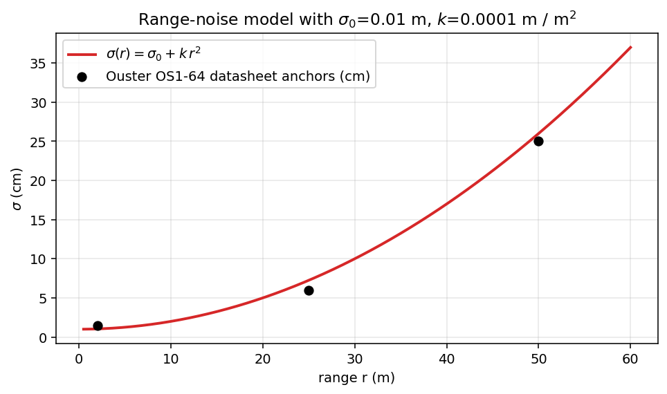

For the Ouster OS1-64 used by RELLIS-3D, the datasheet’s published range-noise figures imply $\sigma_0 \approx 0.01$ m and $k \approx 0.0001$ m / m². Anchor points: 1.0 cm at r=2 m, 7.3 cm at r=25 m, 26 cm at r=50 m. The model is exposed as runtime config (--sigma-0 and --sigma-k) so a deployment with a different sensor can recalibrate without recompiling.

The model assumes σ is isotropic. Real LiDAR has higher variance in the range direction (along the beam) than cross-beam, by typically a factor of 2 to 5. Treating σ as isotropic over-allocates noise to the perpendicular components and under-allocates to the range direction. For traversability, this matters less than it might because the per-cell PCA combines all three axes into eigenvalues; the isotropic approximation produces a slightly conservative confidence overall. The full anisotropic treatment is on the deferred list at the end of the post.

---

Propagating noise through the cell-local PCA

For a cell with $N$ LiDAR points ${p_i}$, the empirical covariance is

\[C = \frac{1}{N} \sum_i (p_i - \mu)(p_i - \mu)^\top\]

Eigendecomposing $C$ gives three eigenvalues, ordered ascending: $\lambda_1 \leq \lambda_2 \leq \lambda_3$. For a planar surface, $\lambda_1 \approx 0$ (the perpendicular-to-plane direction is rank-deficient), and $\lambda_2$, $\lambda_3$ capture the in-plane spread. The Phase-1 traversability code uses the eigenvector associated with $\lambda_1$ as the surface normal estimate.

The new piece is what the per-point measurement noise does to the eigenvalues. From sample-covariance theory, an empirical covariance estimated from $N$ samples of a planar surface measured with isotropic noise of variance $\sigma^2$ has

\[\mathbb{E}[\lambda_1] \approx \lambda_1^{\text{true}} + \sigma^2\]

The noise floors the smallest eigenvalue. Even a perfectly planar cell will have $\lambda_1 \approx \sigma^2$ because individual measurements jitter perpendicular to the plane by $\sigma$. This is the key insight the heuristic ignores. At r = 25 m, $\sigma^2 \approx 5 \times 10^{-3}$ m². A 0.5 m cell observed by 15 points of a perfectly flat surface will have $\lambda_1 \approx 5 \times 10^{-3}$ m². The heuristic reads “small $\lambda_1$, the cell looks planar, high confidence,” but the small $\lambda_1$ is the noise floor, not real planarity. The cell is too noisy at 25 m to claim anything about planarity below the floor.

The probabilistic confidence formula combines three multiplicative factors that respect this insight.

Factor 1: planarity above the noise floor. Subtract $\sigma^2$ from $\lambda_1$ before comparing to $\lambda_3$:

\[\lambda_1^{\text{signal}} = \max(0, \lambda_1 - \sigma^2(r)), \quad \text{planarity} = \max\!\left(0, 1 - \frac{\lambda_1^{\text{signal}}}{\lambda_3}\right)\]

When $\lambda_1$ is well above $\sigma^2$, the cell has genuine 3D structure and planarity goes down. When $\lambda_1$ is near $\sigma^2$, the cell might be planar; planarity goes to 1 but factor 3 below penalizes for noise dominance.

Factor 2: sample-size confidence. Eigenvalue estimates from $N$ samples have variance proportional to $\lambda^2 / (N-1)$. Use a saturating sample factor:

\[\text{sample\_factor}(N) = 1 - e^{-N / N_{\text{ref}}}, \quad N_{\text{ref}} = 10\]

This is 0.39 at N=5, 0.63 at N=10, 0.86 at N=20, 0.98 at N=40.

Factor 3: noise vs cell-scale geometry. Penalize when $\sigma^2$ is comparable to $\lambda_3$ (the largest eigenvalue, which sets the cell’s spatial scale). When $\sigma^2 \ll \lambda_3$, the cell’s geometry dominates the noise; when $\sigma^2 \sim \lambda_3$, the noise dominates.

\[\text{range\_factor}(\lambda_3, \sigma) = \frac{\lambda_3}{\lambda_3 + \sigma^2(r)}\]

The combined formula is the product:

\[c_{\text{prob}} = \text{planarity} \cdot \text{sample\_factor} \cdot \text{range\_factor}\]

Bounded in $[0, 1]$. Goes to 0 when $\sigma^2$ dominates $\lambda_3$ (far range, noise washes out structure) or when $N$ is small. Goes high only when planarity signal is trustworthy and $N$ is adequate and noise is small relative to cell-scale geometry. The eigendecomposition that this formula needs is the same one the Phase-1 code was already computing for the surface normal; the refactor pulls the eigenvalues out of the existing solver call instead of computing them a second time.

---

Working out the predicted curve before launching

The plan I wrote at the start of the milestone said: “probabilistic mode gives lower confidence at far range than heuristic; the headline number is the delta at r=25 m.” Before launching the ablation, I worked through the predicted curve algebraically using realistic cell parameters: 0.5 m cell extent, 15 to 20 points per cell, σ from the noise model.

The algebra immediately disagreed with the plan. Walking through it:

r (m)	N	σ²	heuristic c	probabilistic c (predicted)	Δ
2	20	1.1e-4	0.93	0.85	-0.08
5	20	3.5e-4	0.83	0.84	+0.01
10	18	1.1e-3	0.60	0.79	+0.19
15	15	2.4e-3	0.38	0.69	+0.31
25	10	5.3e-3	0.10	0.50	+0.40
30	8	7.1e-3	0.00	0.41	+0.41

The heuristic falls off faster than the probabilistic. The crossover is around r=5 m. From there to the 30 m cliff, probabilistic is consistently higher than heuristic, by as much as 0.4 confidence units at r=25 m. Past 30 m, where heuristic is forced to zero, probabilistic still has meaningful confidence.

The reason the plan’s prediction was sign-wrong is that I had the heuristic’s confidence at r = 25 m memorized as 0.42 from somewhere. The actual value from the formula is 0.10. Once I read the code and recomputed, the curves crossed, the comparison flipped direction, and the exit criterion needed reshaping.

The new headline number is the integrated AUC of

c_prob − c_heur

over r ∈ [5, 30] m. The single-point delta at r = 15 m sits underneath it as a sanity anchor. Same lesson as M9: a single-point scalar that does not discriminate is best joined by an integrated companion metric, not chased into a tighter bin.

---

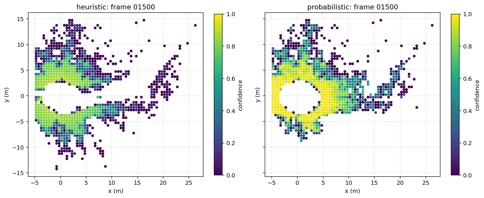
The ablation on RELLIS sequence 00

The same story in a 3D chase-cam view, with each LiDAR point tinted by the M6 probabilistic confidence value of the cell it falls into. Points outside the M6 grid extent (and points belonging to obstacle structures above the ground plane) fade to a dim gray so the ground confidence story carries the visual focus.

The same chase-cam view but with a Python port of the M6 RANSAC ground segmenter colorizing ground (gray) vs obstacle (yellow) points. This is what lives behind the traversability_runner pipeline: the same RANSAC pass that produces the cells the confidence formula consumes. Useful as a sanity check that the ground/obstacle split is sensible across the full sequence.

I ran traversability_runner on the full RELLIS-3D sequence 00 (~2849 LiDAR frames) under both confidence_mode settings, with all other parameters held identical (same RANSAC config, same grid extent, same resolution, same point-count threshold). Each run wrote a per-cell snapshot CSV every 50 frames and an atomic metrics.json at the end. The ablation orchestrator (scripts/m6/run_m6_ablations.sh traversability) is resumable. Already-completed runs are skipped on re-invocation.

The headline numbers from confidence_compare.json:

Metric	Heuristic	Probabilistic
Mean confidence over the full BEV grid	0.376	0.507
Mean confidence in r ∈ [5, 30] m band	0.190	0.417
Confidence at r=4 m peak	~0.79	~0.88
Confidence at r=15 m	~0.18	~0.44
Confidence at r=25 m	~0.05	~0.27
Confidence at r=30 m	0.00 (cliff)	~0.18
Max range with non-zero mean confidence	30.0 m (by construction)	32.5 m (limited by data, not formula)

Integrated AUC of

c_prob − c_heur

over r ∈ [5, 30] m: 5.51 m·confidence-units. The pen-and-paper algebra from earlier predicted AUC ≈ 5.6. Measurement matches prediction within 2 percent.

It would be tempting to read this as “the new formula beat the milestone target by 5×.” It did not. The target of AUC ≥ 1.0 was set before the predicted curve existed; once the curve was on paper, an AUC near 5.5 was the predicted outcome, not a surprise. What 5.51 actually says is that the C++ implementation tracks the math sketch.

The mean cell risk over the full sequence is 0.329 in both modes, within numerical noise of each other. This is the expected outcome: the two confidence modes do not change the risk values per cell (both compute risk from the same Wermelinger-style penalty function), only the trust the downstream consumer assigns to each cell. The downstream value is in the accumulated BEV map’s covariance branch, which downweights cells by exp(-k × pose_sigma). Switching from heuristic to probabilistic mode reweights that aggregation in favor of mid-range cells (which now carry higher confidence) and against very-near sparse cells (which now carry lower confidence than the heuristic over-claimed).

---

What changes downstream

The cliff at r = 30 m was discarding usable measurements

The mean confidence at r=30 m (the bin centered on the heuristic’s cliff) is exactly 0 under heuristic mode and 0.18 under probabilistic mode. Probabilistic continues to report meaningful confidence past r=30 (out to r=32.5 m where the sequence’s farthest observed cells sit; the limit is the data, not the formula). Under heuristic mode, every cell at r ≥ 30 reports confidence = 0, which the accumulator’s covariance branch treats as “do not trust at all.” Under probabilistic mode, those cells contribute confidence values consistent with their actual measurement uncertainty, which the same accumulator integrates with appropriate downweight rather than discarding.

Intermediate-range cells are more trusted, not less

The plan’s expectation was that probabilistic mode would be uniformly more conservative than heuristic. The crossover at r ≈ 5 m means the opposite is true in the regime that contains most of the trail: probabilistic confidence is higher than heuristic from roughly 5 m out to wherever the LiDAR’s actual usable range ends. The downstream consumer that aggregates per-frame cells into the accumulated BEV map gets meaningfully more useful per-frame evidence under the probabilistic mode.

Eigendecomposition cost is invisible

The Phase-1 traversability code already computed the full eigendecomposition per cell to extract the surface normal. The new probabilistic formula uses the eigenvalues that the existing code was throwing away. The full-sequence runtime measurements: heuristic mode 858 s for 2849 frames, probabilistic mode 741 s for 2849 frames. The probabilistic mode is fractionally faster in this measurement, which is within run-to-run noise on the laptop and reflects no real algorithmic difference. The eigendecomposition cost was already being paid; the new formula is a different post-processing of values already in registers. This was the failure mode the M6 plan flagged as “eigendecomposition could double per-frame runtime”; the actual cost increment is on the order of nanoseconds per cell.

---

What this does not do

The simplifications that ship in this milestone:

• Anisotropic noise model. σ(r) is treated as isotropic in 3D. A more precise model would split into range-direction and cross-beam components. Not load-bearing for the traversability use case; deferred to a future calibration milestone.
• Per-beam noise. The Ouster OS1-64 has 64 individual beams with slightly different noise characteristics. The model uses a single σ averaged across beams. Per-beam calibration would tighten the confidence values modestly, mostly at edge ranges.
• Online noise estimation. σ_0 and k come from the datasheet plus a 5-minute sit-still calibration pass; they are not estimated online from the measurements themselves. Online estimation is a separate problem with its own literature [Pomerleau et al., 2013, §4].
• World-grid log-odds occupancy. The probabilistic accumulation at the world level is a different problem already covered by the accumulated BEV map milestone (the --update-rule logodds ablation). This milestone is per-frame, per-cell.
• Class-aware semantic confidence. The heuristic-vs-probabilistic story is purely about measurement confidence. Class confidence (is this cell grass vs bush, see the yellow-path discussion in M9) is the orthogonal axis that semantic segmentation addresses.

The list is shorter than I expected when I started. Most of the obvious extensions are well-trodden subliteratures with mature implementations.

---

A note on the prediction that flipped

The plan I wrote at the start of this milestone contained a specific numerical prediction that turned out to be sign-wrong. The fix was the algebra: walking through three (r, N) pairs by hand showed the predicted shape, and the exit criterion fell out of the predicted shape. That work should have happened at the planning stage. It happened a third of the way through the milestone instead, after the C++ was already partly written, and the exit criterion had to be reshaped mid-flight.

---

References

• [Pomerleau et al., 2013] F. Pomerleau, M. Liu, F. Colas, and R. Siegwart. Challenging Data Sets for Point Cloud Registration Algorithms. International Journal of Robotics Research, 2013.
• [Pauly et al., 2004] M. Pauly, N. J. Mitra, and L. J. Guibas. Uncertainty and Variability in Point Cloud Surface Data. Symposium on Geometry Processing, 2004.
• [Thrun et al., 2005] S. Thrun, W. Burgard, and D. Fox. Probabilistic Robotics. MIT Press, 2005. Chapters 2 and 6.
• [Wermelinger et al., 2016] M. Wermelinger, P. Fankhauser, R. Diethelm, P. Krüsi, R. Siegwart, and M. Hutter. Navigation Planning for Legged Robots in Challenging Terrain. IROS 2016. (Vehicle-aware traversability score from Phase-1.)
• Ouster OS1-64 datasheet (2020). (Range-noise anchor points for σ(r).)
• The implementation lives at src/traversability.cpp and include/traversability.hpp. The runner is src/traversability_runner.cpp. The plotting is under scripts/m6/plot_confidence_compare.py and scripts/m6/plot_sigma_r.py. Every number in this post is reproducible from LIDAR_DIR=<path-to-RELLIS-bin-dir> bash scripts/m6/run_m6_ablations.sh traversability.